Introduction
Over the summer, I undertook the challenge of designing and deploying the development of a self-balancing inverted pendulum (SBIP) robot. The inverted pendulum control problem is a popular example since the inverted pendulum is a naturally unstable system. Only through careful consideration of the controller can the unstable open-loop system become a stable closed-loop system. For those who may be unfamiliar with the inverted pendulum system, imagine trying to balance a pencil that is standing upright on its eraser using only your finger. Naturally, the pencil, in this unstable orientation will begin to fall immediately, so your finger must move in order to move the base of the pencil beneath its center of mass. The documentation of this project will be broken up into several parts to make the content more digestible, and by no means are these posts meant to be rigorous documentation of the project. Starting out on this project, I had several key objectives in mind for what I wanted my robot to be able to achieve:
- Balance indefinitely i.e. be a stable closed-loop system
- Able to resist and dissipate bumps to the pendulum
- Hold a position on the surface i.e. average velocity of the robot is zero over time
My introduction to control theory through my degree focused heavily on applications where PID (proportional-integral-derivative) tuning was an effective means of producing a stable closed-loop system. Traditionally PID is best suited for systems where there is a single input and a single output (SISO). Based on the design objectives defined previously, we can immediately see that since we need to control two outputs (surface position, surface velocity, pendulum position, and pendulum velocity), PID will be an insufficient method to employ unless the design criteria are relaxed.
Mathematical Modelling
After spending some time online researching controller design techniques, I came across a Matlab Controls Tutorial website by Rick Hill of Michigan University which provided detailed explanations of modelling techniques and applications to a variety of mechanical control problems, including the inverted pendulum (IP) problem. The modelling analysis provided is quite common, in respect to the IP, so I will only pull out the important points for presentation here.
We start off with the free body diagram for the assembly. The diagram consists of the pendulum, which is modelled simply as a rod in this case, as well as a cart to which the pendulum is affixed. Force is applied at the cart to counteract motion of the pendulum away from an upright position. For example, if the pendulum begins falling to the left, the cart will move to the left creating a moment about the center of the pendulum and causing the pendulum to return to an upright position.
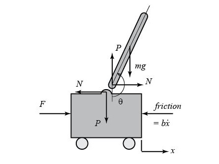
There are two nonlinear differential equations required to accurately describe the motion of the IP. The first equation is found by summing the horizontal forces in the cart and then the pendulum. Following this, one equation is substituted into the other to arrive at:

Similarly, the second equation of motion can be found by summing the forces perpendicular to the axis of the pendulum. The resulting equation is

Linearization
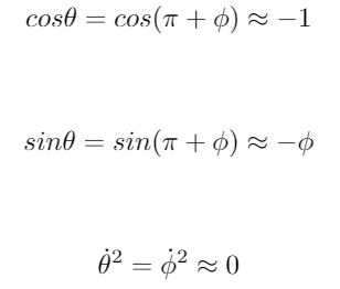
The last step is to linearize the two equations of motion. The equations must be linearized since the techniques used to design the controller for the system must be applied to a linear-time-invariant system in order to be valid. The linearization will be valid within error as long as the pendulum does not deviate further then 20 degrees from the point of linearization. Beyond that point, the error will begin to become too great and the system could become unstable despite the control action applied. Referring to Figure 1, the angle of the pendulum (θ) in the upright position is at π degrees. A deviation of φ degrees affects the pendulum according to θ = π + φ. The following approximations are substituted into the two nonlinear equations of motion,
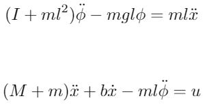
The resulting force equations for the cart and pendulum after the linearization has been applied is shown below. Note that the force F has been replaced with u to indicate controller action.
State-Space Equations
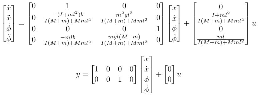
In order to efficiently deal with the multiple outputs (pendulum angle, pendulum angular velocity, cart position, cart velocity) from the system and the single input (control force, u), the equations must be converted to a state space model. Rearranging the equations to a set of first order differential equations, the state space model can be represented as
Matlab State-Space Modelling
The set of state-space equations must also be converted into Matlab code in order to perform simulations of the open-loop and closed-loop systems. Further on in this post, it is shown how weightings of the state variables are selected in the controller to obtain a closed-loop response of the system that satisfies the design requirements. The Matlab code below was grabbed from the Matlab Controls Tutorial site mentioned previously in the post. Parameter values for the model are included in the code but are arbitrary until the robot is constructed. Once the robot is fully assembled, the moment of inertia and the center of mass can be computed, the mass of both the cart and pendulum can be measured, and these parameters can be factored into the model.
M = .5; % mass of cart in kg
m = 0.2; % mass of pendulum in kg
b = 0.1; % drag coefficient
I = 0.006; % moment of inertia in kg-m^2
g = 9.8; % gravitational acceleration
l = 0.3; % length to pendulum center of mass

p = I*(M+m)+M*m*l^2;

A = [0      1              0           0;
     0 -(I+m*l^2)*b/p  (m^2*g*l^2)/p   0;
     0      0              0           1;
     0 -(m*l*b)/p       m*g*l*(M+m)/p  0];
B = [ 0; (I+m*l^2)/p; 0; m*l/p];
C = [1 0 0 0; 0 0 1 0];
D = [ 0; 0];

states = {'x' 'x_dot' 'phi' 'phi_dot'};
inputs = {'u'};
outputs = {'x'; 'phi'};

sys_ss = ss(A,B,C,D, 'statename',states, 'inputname',inputs, 'outputname',outputs);

Ts = 1/100;

sys_d = c2d(sys_ss,Ts,'zoh')
Matlab Closed-loop Modelling
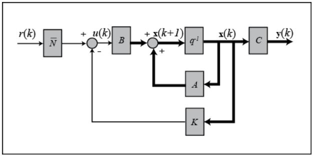
Now that a mathematical model has been created that represents the IP, it is time to set up the simulation and close the feedback loop. Full-state feedback of the cart position, cart velocity, pendulum angle, and pendulum angular velocity is used to inform the control action taken by the controller and motors. In full state feedback, a vector of gains, K, where each element corresponds to a state of the system, is multiplied with the current state vector to output the force required by the motors for the current timestep.
The optimal gain matrix, K, can be determined using a technique known as LQR (linear quadratic regulation). LQR consists of a Q matrix, which is the state-cost matrix, and an R matrix, which is the performance matrix. This method is not completely autonomous as the designer is still required to specify the cost values in the Q matrix, however, it is quite easy iterate by selecting Q-matrix values until the desired response is achieved. The following Matlab code can be added to the previous code to simulate the IP system under closed-loop control.
A = sys_d.a;
B = sys_d.b;
C = sys_d.c;
D = sys_d.d;
Q = C'*C;*
Q(1,1) = 5000; % cart position
Q(3,3) = 100; % pendulum angle
R = 1;
[K] = dlqr(A,B,Q,R)

Ac = [(A-B*K)];
Bc = [B];
Cc = [C];
Dc = [D];

states = {'x' 'x_dot' 'phi' 'phi_dot'};
inputs = {'r'};
outputs = {'x'; 'phi'};

Nbar = -62; % precompensator
sys_cl = ss(Ac,Bc*Nbar,Cc,Dc,Ts, 'statename',states, 'inputname',inputs, 'outputname',outputs);

t = 0:0.01:5;
r =0.2*ones(size(t));
[y,t,x]=lsim(sys_cl,r,t);
[AX,H1,H2] = plotyy(t,y(:,1), t,y(:,2), 'plot');
set(get(AX(1),'Ylabel'), 'String', 'cart position (m)')
set(get(AX(2),'Ylabel'), 'String', 'pendulum angle (radians)')
title('Step Response with Digital LQR Control')
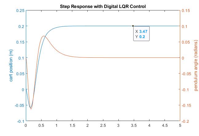
The first thing to note about this code is that the disturbance used in this case is a command for the cart to move 0.2 m from a position of 0.0 m. The second thing to note is that there is an Nbar term included in the code. This term is the precompensator and must be tuned for each system, otherwise the cart-pendulum system will not go to the commanded position. This is due to the fact that the full state feedback system does not directly compare states to their desired value. For example, if a cart position of 0.2 m is commanded, without the tuned precompensator value, the cart may go to any other value than 0.2 m. Through trial and error, the precompensator value is selected such that the final cart position matches the commanded position within a defined uncertainty. Figure 2 displays the output of the Matlab simulation once the precompensator value has been tuned.
With the full-state feedback set up, as well as the precompensator, the schematic for the control system and the open-loop plant takes the following form:
