Introduction
For any power system to operate under normal balanced three-phase steady state conditions, it must be ensured that the generation is sufficient for the load on the system, that bus voltages do not deviate significantly from rated values, generators operate within their real and reactive power limits, and transmission lines and transformers do not become overloaded. The basic tool to investigate satisfaction of these criteria is a power flow calculation for given power system parameters. In this post, we will be looking into power flow solutions utilizing the Newton Raphson method and briefly reviewing code I developed in Matlab to implement the power flow solution method.
The Math
As we start, I should note I have drawn from the textbook Power System Analysis and Design by D.Glover, M. Sarma, T. Overbye to aid in the explanation of the calculation and for the formula images. There are a couple different pieces that are required in order to begin this calculation. For each bus in the system, we need to set up variables for the voltage (V), voltage angle (delta), real power (P), and reactive power (Q). For the calculation, the variables are rolled into the vectors shown below. Depending on the types of buses being considered, some of these variables could be omitted but for now we are assuming all are required.
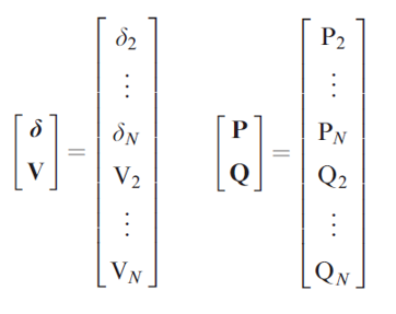
Where V, P, and Q are in per-units but the voltage angle, delta, is in radians. Note, that the vector elements are numbered from 2 to N where N is the number of buses in the power system and 1 is omitted because it would refer to the slack bus (or the main grid bus) for which the voltage and voltage angle are already known (1.0 + j0.0 p.u.).
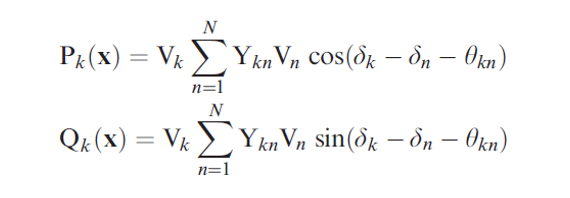
Next, the real and reactive power for bus k for k = 2, 3, ..., N can be calculated according to the equations below utilizing the values for V and delta according the values of the latest iteration for these variables. For the first iteration, these would be initial guesses of these values.
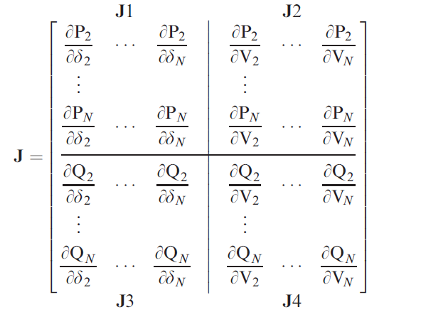
The last major piece is the Jacobian matrix for the power system. It is shown below and split into four different regions, J1 to J4.
For instances where n does not equal k, J1 to J4 can be calculated as
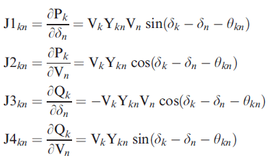
and for instances where n does equal k, the equations below can be used
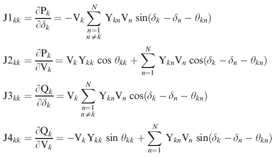
where k, n = 2, 3, ..., N.
With these three different pieces introduced we can move to describing the procedure for the calculation, which is broken up into four steps. Starting from initial guesses for the bus voltages and bus voltage angles,

step 1 is to compute a comparison of the real and reactive power at bus k by calculating the difference between the defined real and reactive power for bus k and the real and reactive power at bus k as determined by the equations from Figure 2. This result could be called the real and reactive power variance vector.

Step 2 is next and requires the use of the equations from figures 4 and 5 to compute the Jacobian matrix in figure 3. In practice, step 1 and step 2 can actually be swapped if desired since the steps do not depend on the other to proceed with the calculation. Step 3 requires setting up the Jacobian matrix and real and reactive power variance vector in an Ax = b matrix equation format to determine the vector for the bus voltage and voltage angle variances, as shown below.

The matrix equation can be solved using Gaussian elimination and back substitution. Lastly, for step 4, the bus voltage and voltage angle variance vector is used with the current iteration vector, iteration i, for the bus voltages and voltage angles to determine the bus voltages and voltage angles for use in the next iteration, iteration i+1.

The iteration i+1 values are then used to start the process all over again and continues either until a particular number of iterations have elapsed or some solution uncertainty criteria has been reached. A common criteria is called a power mismatch and defines the magnitude of the variances in the real and reactive power variance vector.
The Code
The code I developed to implement the power flow solution by the Newton Raphson technique is shown in the code block below. It is broken up into three sections: Inputs, Code, and Results. Under the input section, the values that describe the power system to be analyzed are entered. These are the values for bus voltage, bus voltage angle, real and reactive power, and the bus admittance matrix for the power system which describes how the buses are connected. The last value to edit is the number of iterations to run the procedure, shown a little lower down. The code currently has is set to run 4 times (Iteration = 1:4).
Assuming the values for the scenario have been entered correctly, then hitting run in Matlab will execute the code and at the end of each iteration Matlab will report the results of the calculation as shown at the bottom of the code under Iteration Results. I have entered the inputs already for a question from Power System Analysis and Design which features two buses with defined real and reactive power requirements (P-Q buses or load buses).
  clear

  %%%%%%%%%%%%%%%%%%%%%%%%%%%%%%%%%%%%%%%%%%%%%%%%%%%%%%%%%%%%%%%%%%%%%%%%
  %                          Scenario Inputs                             %
  %%%%%%%%%%%%%%%%%%%%%%%%%%%%%%%%%%%%%%%%%%%%%%%%%%%%%%%%%%%%%%%%%%%%%%%%

  % Enter voltage magnitudes in per-unit. Element 1 is always the slack bus.
  % Enter rows for each bus in the system with the guess for the voltage.
  V = [1;
      1;
      1];

  % Enter the angles for the bus voltages in radians. Element 1 is always
  % for the slack bus. Must have the same number of rows as vector V and are
  % the initial guesses for the system.
  Delta = [0;
      0;
      0];

  % Enter Ybus in per-unit.
  Ybus = [-10*1i 5*1i 5*1i;
          5*1i -10*1i 5*1i;
          5*1i 5*1i -10*1i];

  % Enter powers as negative when drawing on the power system and
  % positive when adding to the system for both P and Q. Enter in per-unit.
  % First entry corresponds to the first load bus after the slack bus i.e.
  % the slack bus is not included in these vectors.
  P_i = [-1;
      -1.5];
  Q_i = [-0.5;
      -0.75];

  %%%%%%%%%%%%%%%%%%%%%%%%%%%%%%%%%%%%%%%%%%%%%%%%%%%%%%%%%%%%%%%%%%%%%%%%
  %                            Code Begins                               %
  %%%%%%%%%%%%%%%%%%%%%%%%%%%%%%%%%%%%%%%%%%%%%%%%%%%%%%%%%%%%%%%%%%%%%%%%


  % Initialize arrays to hold the results of jacobian matrix calculations
  J1 = zeros(size(V,1)-1,size(V,1)-1);
  J2 = zeros(size(V,1)-1,size(V,1)-1);
  J3 = zeros(size(V,1)-1,size(V,1)-1);
  J4 = zeros(size(V,1)-1,size(V,1)-1);

  % Initialize P and Q vectors
  P = P_i;
  Q = Q_i;

  for Iteration = 1:4
      % compute n equals k entries for Jacobian matrices
      for k = 2:size(V,1) % don't need to count slack bus which is always in the no. 1 slot
          % Compute J1 values for n equal to k
          J1kk_sum = 0;
          for n = 1:k-1
              J1kk_sum = J1kk_sum + abs(Ybus(k,n))*V(n)*sin(Delta(k)-Delta(n)-angle(Ybus(k,n)));
          end
          for n = k+1:size(V,1)
              J1kk_sum = J1kk_sum + abs(Ybus(k,n))*V(n)*sin(Delta(k)-Delta(n)-angle(Ybus(k,n)));
          end
          J1kk = -1*V(k)*J1kk_sum;
          J1(k-1,k-1) = J1kk;
      end

      for k = 2:size(V,1) % don't need to count slack bus which is always in the no. 1 slot
          % Compute J2 values for n equal to k
          J2kk_sum = 0;
          for n = 1:size(V,1)
              J2kk_sum = J2kk_sum + abs(Ybus(k,n))*V(n)*cos(Delta(k)-Delta(n)-angle(Ybus(k,n)));
          end
          J2kk = J2kk_sum + V(k)*abs(Ybus(k,k))*cos(angle(Ybus(k,k)));
          J2(k-1,k-1) = J2kk;
      end

      for k = 2:size(V,1) % don't need to count slack bus which is always in the no. 1 slot
          % Compute J3 values for n equal to k
          J3kk_sum = 0;
          for n = 1:k-1
              J3kk_sum = J3kk_sum + abs(Ybus(k,n))*V(n)*cos(Delta(k)-Delta(n)-angle(Ybus(k,n)));
          end
          for n = k+1:size(V,1)
              J3kk_sum = J3kk_sum + abs(Ybus(k,n))*V(n)*cos(Delta(k)-Delta(n)-angle(Ybus(k,n)));
          end
          J3kk = V(k)*J3kk_sum;
          J3(k-1,k-1) = J3kk;
      end

      for k = 2:size(V,1) % don't need to count slack bus which is always in the no. 1 slot
          % Compute J4 values for n equal to k
          J4kk_sum = 0;
          for n = 1:size(V,1)
              J4kk_sum = J4kk_sum + abs(Ybus(k,n))*V(n)*sin(Delta(k)-Delta(n)-angle(Ybus(k,n)));
          end
          J4kk = J4kk_sum - V(k)*abs(Ybus(k,k))*sin(angle(Ybus(k,k)));
          J4(k-1,k-1) = J4kk;
      end

      % Calculate the Jacobian matrix values for where n does not equal k

      % Compute J1 values for n not equal to k
      for k = 2:size(V,1)
          J1kn_sum = 0;
          for n = 2:k-1
              J1kn_sum = V(k)*abs(Ybus(k,n))*V(n)*sin(Delta(k)-Delta(n)-angle(Ybus(k,n)));
              J1(k-1,n-1) = J1kn_sum;
          end
          for n = k+1:size(V,1)
              J1kn_sum = V(k)*abs(Ybus(k,n))*V(n)*sin(Delta(k)-Delta(n)-angle(Ybus(k,n)));
              J1(k-1,n-1) = J1kn_sum;
          end
      end

      % Compute J2 values for n not equal to k
      for k = 2:size(V,1)
          J2kn_sum = 0;
          for n = 2:k-1
              J2kn_sum = V(k)*abs(Ybus(k,n))*cos(Delta(k)-Delta(n)-angle(Ybus(k,n)));
              J2(k-1,n-1) = J2kn_sum;
          end
          for n = k+1:size(V,1)
              J2kn_sum = V(k)*abs(Ybus(k,n))*cos(Delta(k)-Delta(n)-angle(Ybus(k,n)));
              J2(k-1,n-1) = J2kn_sum;
          end
      end

      % Compute J3 values for n not equal to k
      for k = 2:size(V,1)
          J3kn_sum = 0;
          for n = 2:k-1
              J3kn_sum = -1*V(k)*abs(Ybus(k,n))*V(n)*cos(Delta(k)-Delta(n)-angle(Ybus(k,n)));
              J3(k-1,n-1) = J3kn_sum;
          end
          for n = k+1:size(V,1)
              J3kn_sum = -1*V(k)*abs(Ybus(k,n))*V(n)*cos(Delta(k)-Delta(n)-angle(Ybus(k,n)));
              J3(k-1,n-1) = J3kn_sum;
          end
      end

      % Compute J4 values for n not equal to k
      for k = 2:size(V,1)
          J4kn_sum = 0;
          for n = 2:k-1
              J4kn_sum = V(k)*abs(Ybus(k,n))*sin(Delta(k)-Delta(n)-angle(Ybus(k,n)));
              J4(k-1,n-1) = J4kn_sum;
          end
          for n = k+1:size(V,1)
              J4kn_sum = V(k)*abs(Ybus(k,n))*sin(Delta(k)-Delta(n)-angle(Ybus(k,n)));
              J4(k-1,n-1) = J4kn_sum;
          end
      end
      J = [J1 J2
          J3 J4];

      % Compute P and Q vectors for ith iteration
      for k = 2:size(V,1)
          P_sum = 0;
          for n = 1:size(V,1)
              P_sum = P_sum + abs(Ybus(k,n))*V(n)*cos(Delta(k)-Delta(n)-angle(Ybus(k,n)));
          end
          P_k = V(k)*P_sum;
          P(k-1) = P_k;
      end

      for k = 2:size(V,1)
          Q_sum = 0;
          for n = 1:size(V,1)
              Q_sum = Q_sum + abs(Ybus(k,n))*V(n)*sin(Delta(k)-Delta(n)-angle(Ybus(k,n)));
          end
          Q_k = V(k)*Q_sum;
          Q(k-1) = Q_k;
      end

      % Compute P-P(i) and Q-Q(i)...
      delta_p = P_i - P;
      delta_q = Q_i - Q;
      delta_y = [delta_p;
          delta_q];

      % Converting variables for use in back substitution code
      A = J;
      b = delta_y;

      % Gaussian elimination and back substitution code
      [row,col] = size(A);
      n = row;
      x = zeros(size(b));
      for k = 1:n-1
        for i = k+1:n
           xMultiplier = A(i,k) / A(k,k);
           for j=k+1:n
              A(i,j) = A(i,j) - xMultiplier * A(k,j);
           end
           b(i, :) = b(i, :) - xMultiplier * b(k, :);
        end
      % There is a missing "end" ?!
          % backsubstitution:
          x(n, :) = b(n, :) / A(n,n);
          for i = n-1:-1:1
              summation = b(i, :);
              for j = i+1:n
                  summation = summation - A(i,j) * x(j, :);
              end
              x(i, :) = summation / A(i,i);
          end
      end

      x; % resultant deltas in bus angles and bus voltage magnitudes

      delta_Delta = x(1:size(x,1)/2);
      delta_V = x((size(x,1)/2)+1:size(x,1));

      % calculating new bus voltages and angles based on deltas calculated
      for k = 2:size(V,1)
          Delta(k) = Delta(k) + delta_Delta(k-1);
          V(k) = V(k) + delta_V(k-1);
      end

  %%%%%%%%%%%%%%%%%%%%%%%%%%%%%%%%%%%%%%%%%%%%%%%%%%%%%%%%%%%%%%%%%%%%%%%%
  %                          Iteration Results                           %
  %%%%%%%%%%%%%%%%%%%%%%%%%%%%%%%%%%%%%%%%%%%%%%%%%%%%%%%%%%%%%%%%%%%%%%%%

      Iteration
      Delta;
      Delta_degrees = Delta*180/pi;
      V;
      P;
      Q;
      J;

      output = [V Delta_degrees]
  end
After running the code, the results appear as shown below
  >> Newton_Raphson_Power_Flow_Solver_Q6_42

  Iteration =
       1
  output =

      1.0000         0
      0.8833  -13.3690
      0.8667  -15.2789


  Iteration =
       2
  output =

      1.0000         0
      0.8145  -16.4110
      0.7882  -19.2756


  Iteration =
       3
  output =

      1.0000         0
      0.8019  -16.9610
      0.7731  -20.1021


  Iteration =
       4
  output =

      1.0000         0
      0.8015  -16.9811
      0.7725  -20.1361
The first bus or row in each of the tables is the slack bus which stays at a voltage of 1.0 pu and 0 degrees by definition. Following the slack bus in the tables are buses 2 and 3. At iteration 4, we find bus 2 has a voltage of 0.8015 pu with an angle of -16.9811 degrees and bus 3 has a voltage of 0.7725 pu and an angle of -20.1361 degrees. Since the code was set up for a question from the Power System Analysis and Design textbook mentioned earlier, we can compare the results to the answer book in the textbook to verify the correct result was achieved.

Closing Remarks
As this code is designed, it requires the user to have a good idea of their bus admittance matrix for the power system which may require the user to perform an extra step and also assumes that only load buses or P-Q buses are being present. Modifications would be required to accommodate the inclusion of P-V buses or rather buses with a defined real power and voltage such as those that would be connected to generators in a power system. Given these limitations, the logical next step would be to further develop the code to be capable of computing the bus admittance matrix and also be able to solve systems with more than just P-Q buses. Perhaps in the future!